Causal Mediation Analysis for Functional Data
Xi (Rossi) LUO
Health Science Center
School of Public Health
Dept of Biostatistics
and Data Science
ABCD Research Group

July 12, 2024
Funding: NIH R01MH126970, R01EB022911
Collaborators

Yi Zhao
Indiana Univ
Michael Sobel
Columbia Univ

Johns Hopkins Univ

Brian Caffo
Johns Hopkins Univ
Slides viewable on web:
bit.ly /fmjcsds
fMRI Experiments
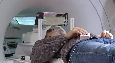
- Task fMRI: performs tasks under brain scanning
-
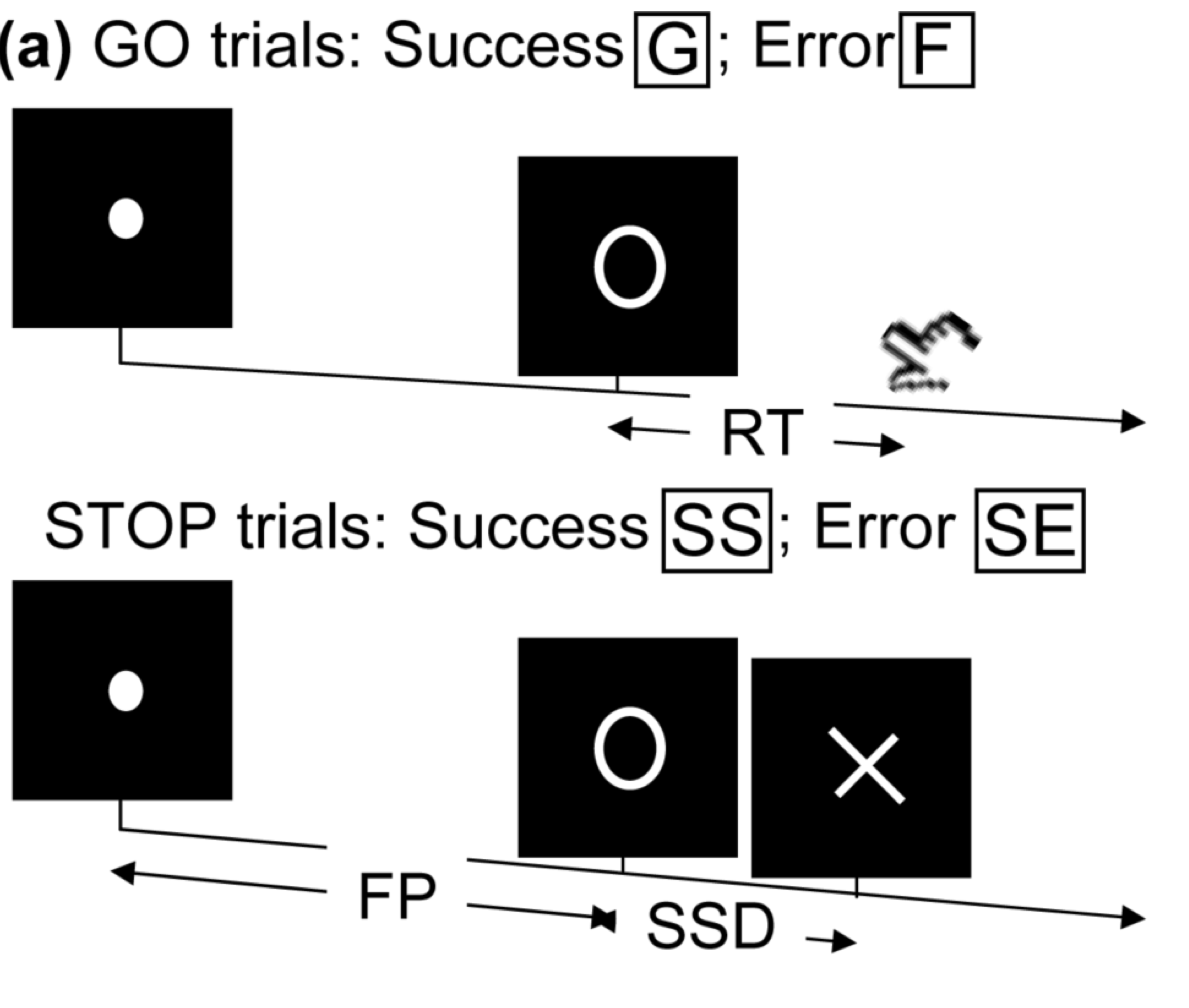
Randomized stop/go task:- press button if "go";
- withhold pressing if "stop"
- Not resting-state: "do nothing" during scanning
fMRI data: blood-oxygen-level dependent (BOLD) signals from each
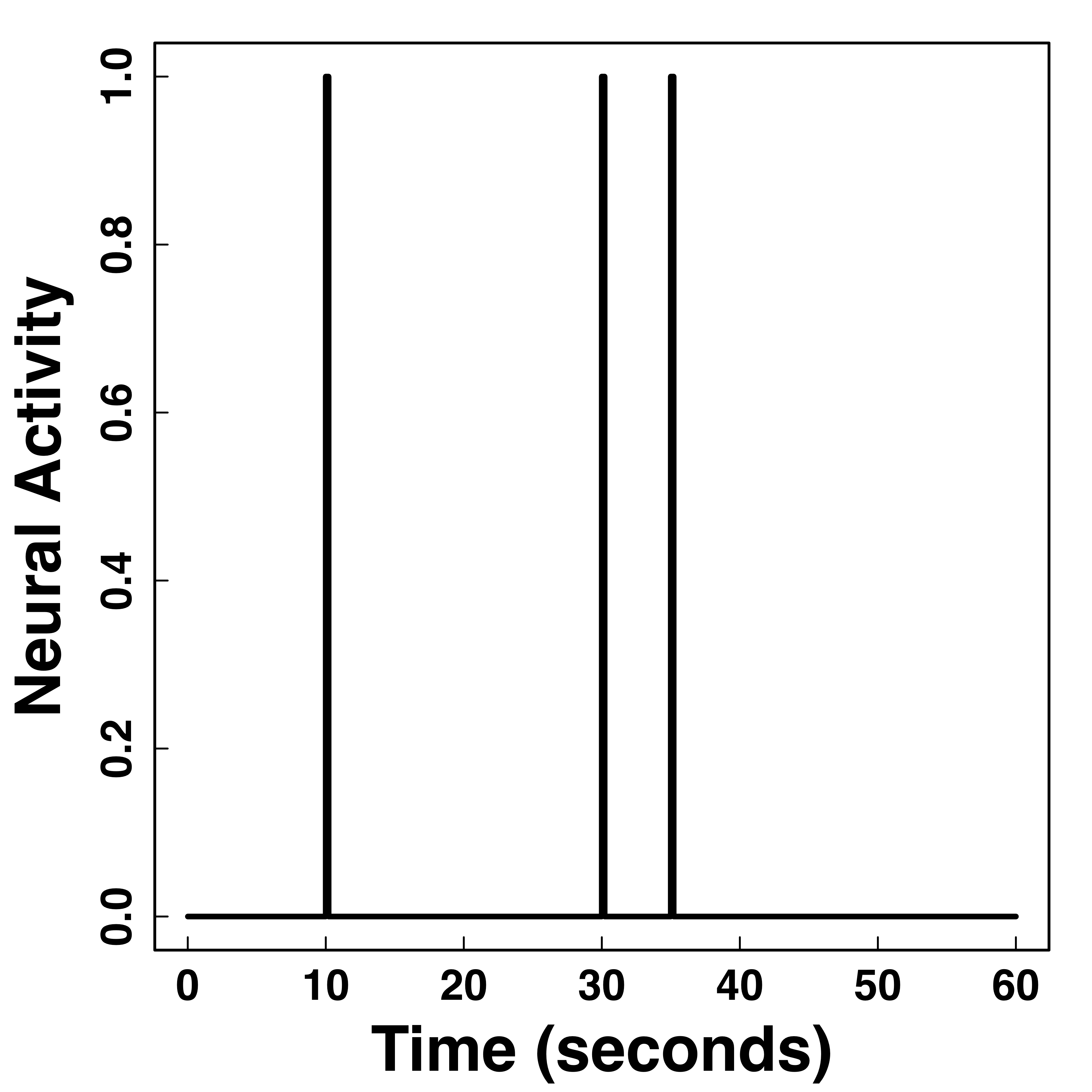
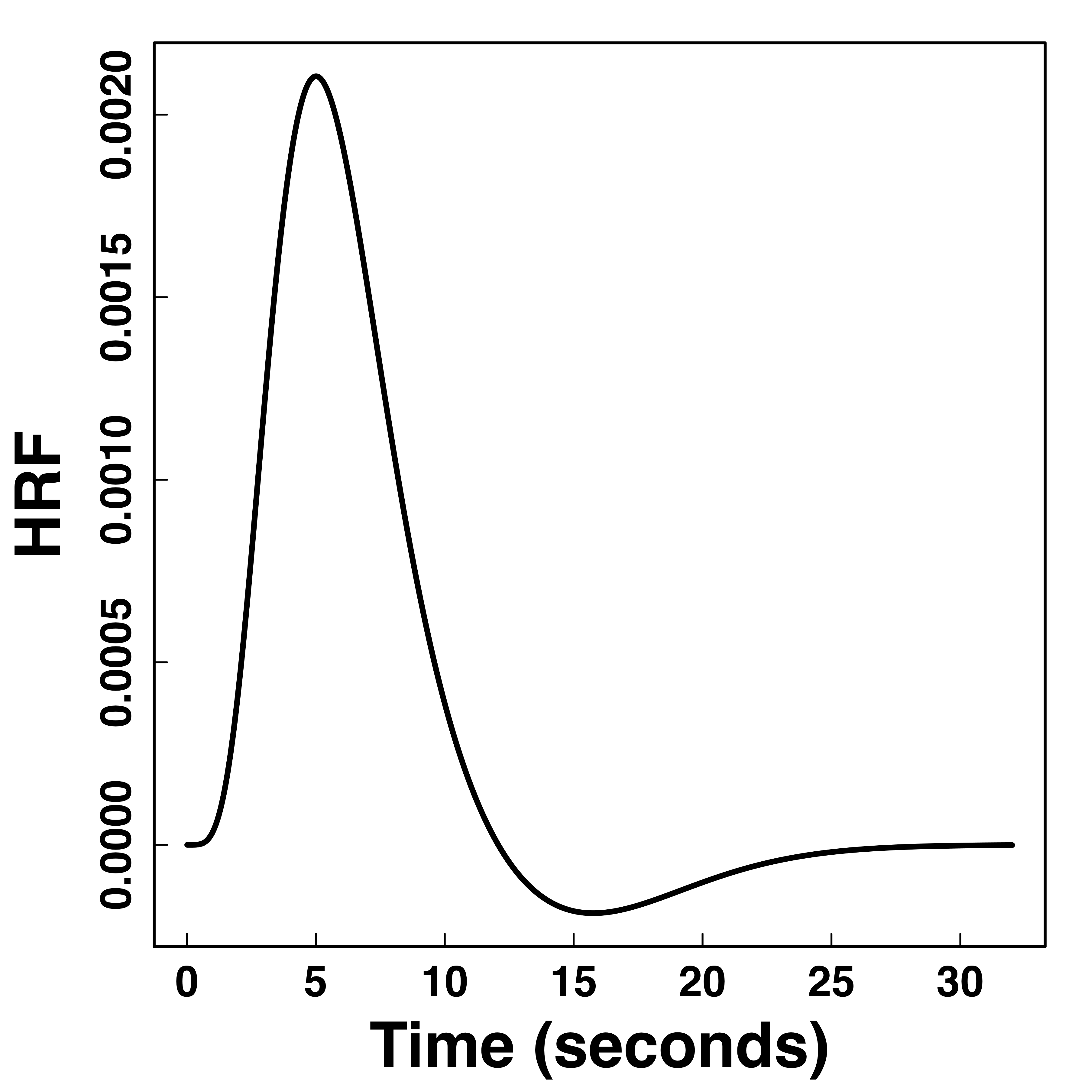
Functional Data
Hemodynamic Response Function (HRF)
 $\otimes$
 $=$
$=$
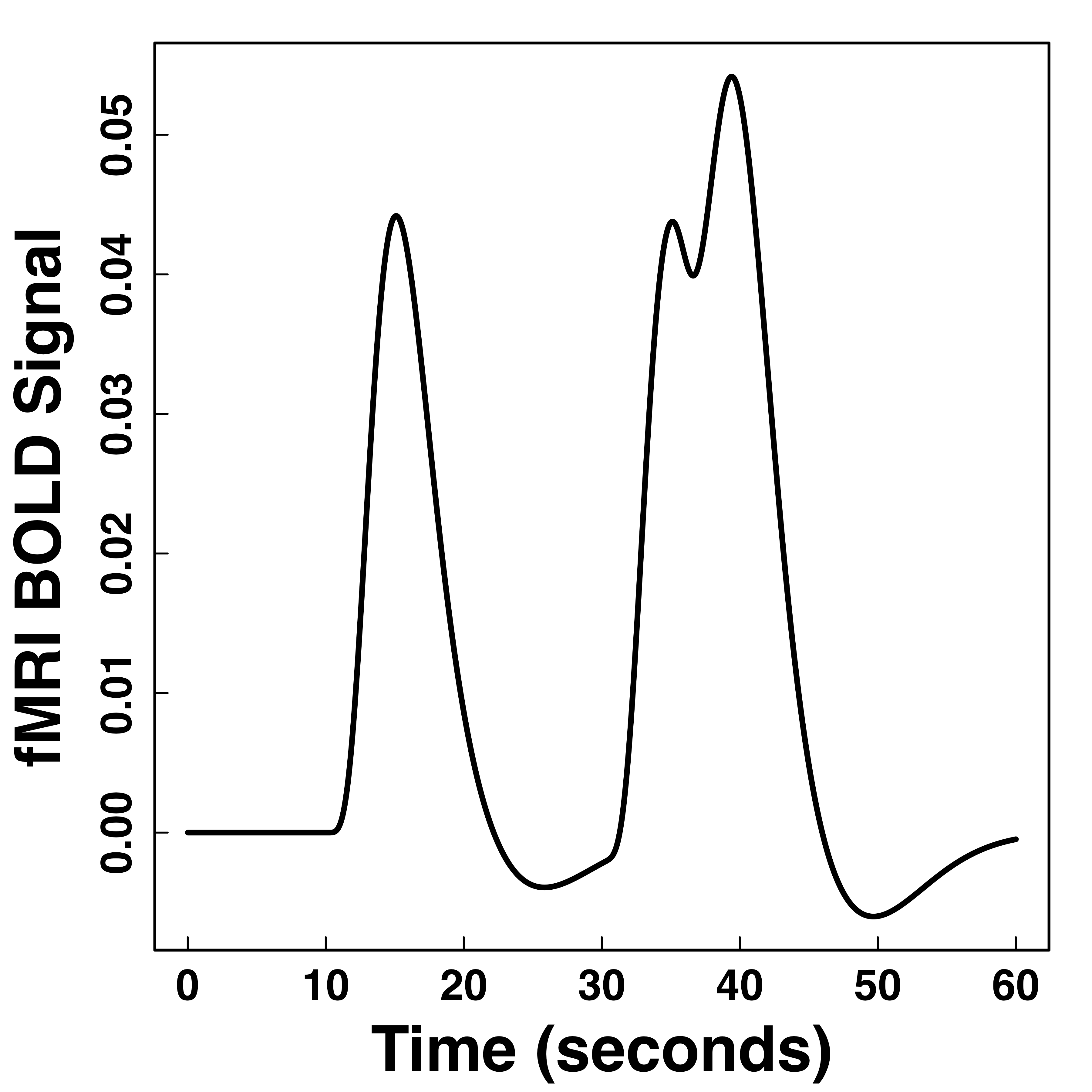
Stimulus sequence convolutions are
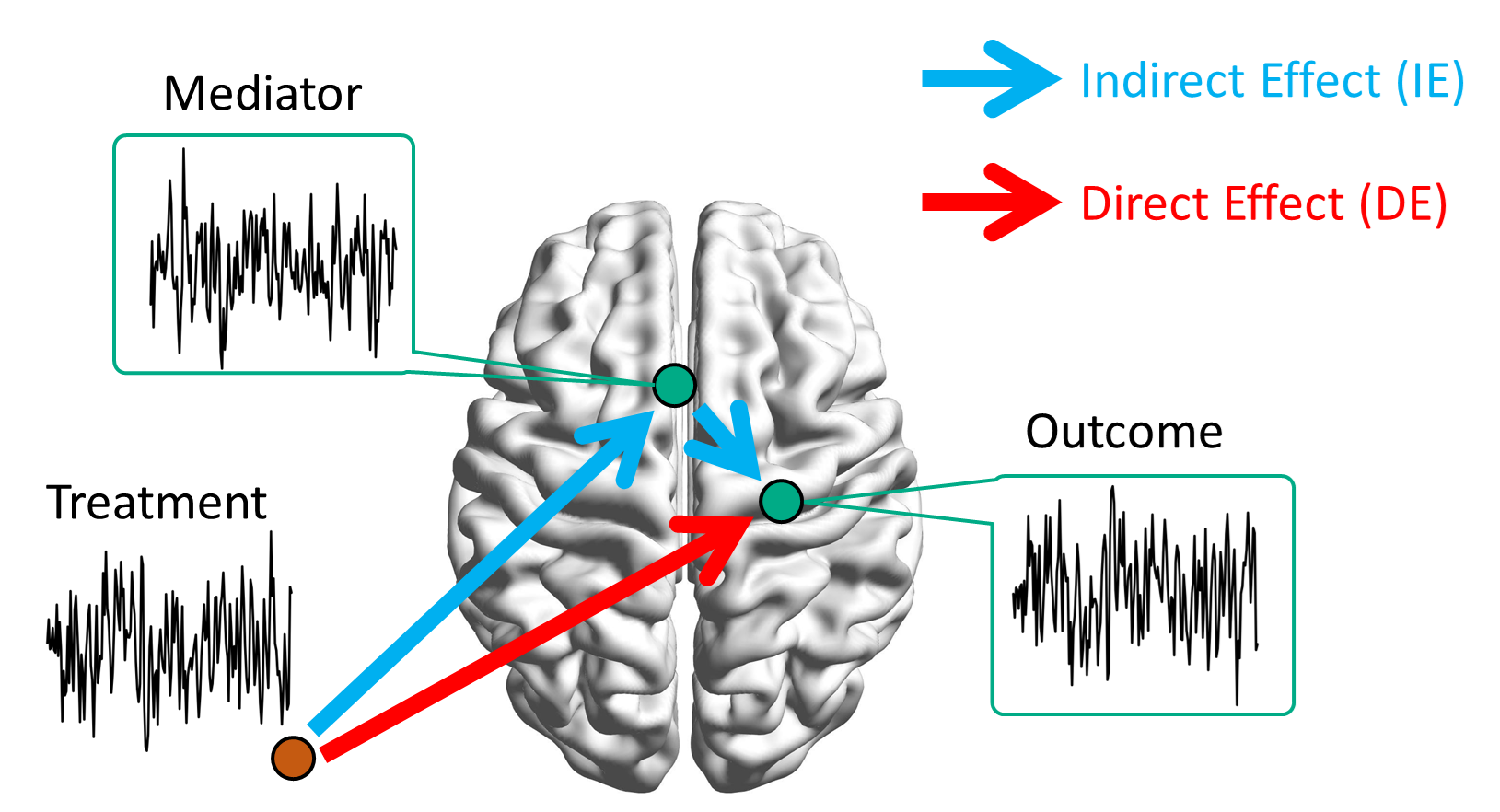
Functional Mediation: Conceptual
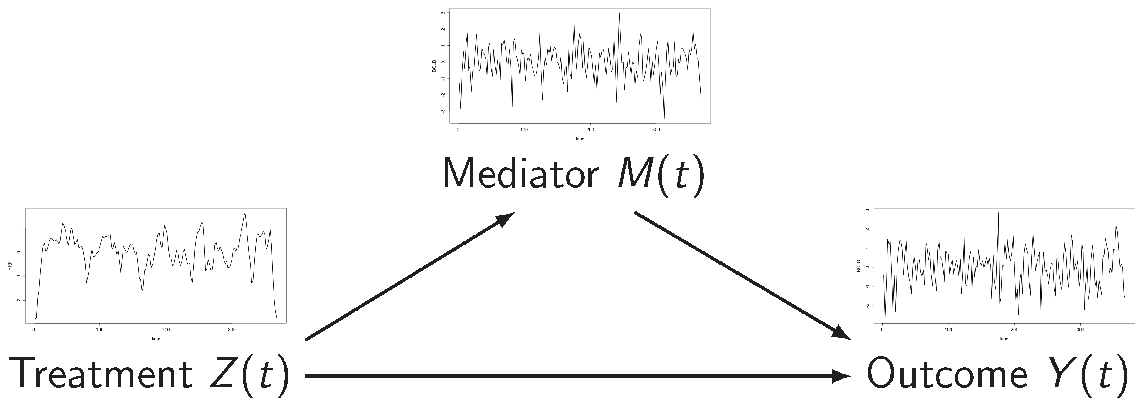
All are functional data
Arrows represent quantifiable causal effects (curves)
Literature Review
- Mediation is an active area
- Classical mediation deals with scalar variables Baron and Kenny, 1986
- Recent work on sparse longitudinal data Zheng and van der Laan, 2017; VanderWeele and Tchetgen Tchetgen, 2017
- Multilevel data Zhao and Luo, 2023
- High dimensional settings Zhao and Luo, 2022
- Intersection with functional/time series models
- Parametric time series models Zhao and Luo, 2019
- Sparse and irregular longitudinal data Zeng and others, 2021
- Functional mediation with
scalar treatments and outcomes Lindquist, 2012 - Spatial-temporal mediator with
scalar variables Jiang and Colditz, 2023; Xu and Kang, 2023 - This work:
functional treatments,functional mediators, andfunctional outcomes
Causal Estimands and Assumptions
Notations
- Let $Z_{t}\in\mathcal{D}_{t}^{z}$, $M_{t}\in\mathcal{D}_{t}^{m}$, and $Y_{t}\in\mathcal{D}_{t}^{y}$
observed at time $t \in [0, T].$ - Let $\bar{Z}_{[s,t]}=\{Z_{u}:s\leq u\leq t\}$, similarly for $\bar{M}_{[s,t]}$, and $\bar{Y}_{[s,t]}$.
- When $s=0$, write $\bar{Z}_{[0,t]}\equiv\bar{Z}_{t}$, similarly for $\bar{M}_{[0,t]}$ and $\bar{Y}_{[0,t]}$.
- Let $M_{t}(\bar{z}_{T})$ and $Y_{t}(\bar{z}_{T})\equiv Y_{t}(\bar{z}_{T},\bar{M}_{T}(\bar{z}_{T}))$ denote, respectively, the potential values of the mediator and outcome at time $t$ when the treatment path is set to $\bar{z}_{T}$
and let $Y_{t}(\bar{z}_{T},\bar{m}_{T})$ denote the
potential value of the outcome at time $t$ when the treatment path is set to $\bar{z}_{T}$ and the mediator path to $\bar{m}_{T}$.
Total Effect, Indirect/Direct Effects
$$ \begin{align} \mathrm{TE}(t;\bar{z}_{t},\bar{z}_{t}^{*}) =& \mathbb{E}\left\{Y_{t}(\bar{z}_{t},\bar{M}_{t}(\bar{z}_{t}))-Y_{t}(\bar{z}_{t}^{*},\bar{M}_{t}(\bar{z}_{t}^{*}))\right\} \\ =& \mathbb{E}\left\{Y_{t}(\bar{z}_{t},\bar{M}_{t}(\bar{z}_{t}))-Y_{t}(\bar{z}_{t},\bar{M}_{t}(\bar{z}_{t}^{*}))\right\} +\\ &\mathbb{E}\left\{Y_{t}(\bar{z}_{t},\bar{M}_{t}(\bar{z}_{t}^{*}))-Y_{t}(\bar{z}_{t}^{*},\bar{M}_{t}(\bar{z}_{t}^{*}))\right\} \nonumber \\ =& \mathrm{TIE}(t;\bar{z}_{t},\bar{z}_{t}^{*}) + \mathrm{PDE}(t;\bar{z}_{t},\bar{z}_{t}^{*}). \end{align} $$- Total effect (TE) of treatment
path $\bar{z}_{t}$ versus path $\bar{z}_{t}^{*}$ on $Y_{t}$ - These are functional versions where funtional potential outcomes depend on functional treatment paths
Assumptions
- A1: $\Pr(\bar{Z}_{T} \in \tilde{\mathcal{D}}_{T}^{z}) > 0$; for any Borel measurable subset $\tilde{\mathcal{D}}^{zm}_{T}$ of $\bar{\mathcal{D}}^{zm}_{T}$ with positive measure, $\Pr((\bar{Z}_{T}, \bar{M}_{T}) \in \tilde{\mathcal{D}}_{T}^{zm}) > 0$.
- A2: For all $\bar{z}_{T}\in \bar{\mathcal{D}}^{z}_{T}$, $$ \begin{equation} \label{eq:causal_assump1a} \bar{Y}_{t}(\bar{z}_{T},\bar{M}_{T}(\bar{z}_{T}))~\bot~\bar{Z}_{T}, \end{equation} $$ and for all $(\bar{z}_{T}, \bar{m}_{T}) \in \bar{\mathcal{D}}_{T}^{zm}$, $$ \begin{equation}\label{eq:causal_assump1b} \bar{Y}_{T}(\bar{z}_{T},\bar{m}_{T})~\bot~\bar{Z}_{T}, \end{equation} $$
- A3: For all $t\in[0,T]$ and ($\bar{z}_{t}, \bar{m}_{t}) \in \bar{\mathcal D}_{t}^{zm}$, $$ \begin{equation}\label{eq:causal_assump2} Y_{t}(\bar{z}_{t},\bar{m}_{t})~\bot~\bar{M}_{t}(\bar{z}_{t}) \mid \bar{Z}_{t}. \end{equation} $$
- A4: For all $\bar{z}_{T}\in\bar{\mathcal{D}}_{T}^{z}$, $$ \begin{equation}\label{eq:causal_assump3} \bar{M}_{T}(\bar{z}_{T})~\bot~\bar{Z}_{T}. \end{equation} $$
- A5: For all $t\in[0,T]$ and triples $(\bar{z}_{t}, \bar{z}^{*}_{t}, \bar{m}_{t}) \in \bar{\mathcal{D}}_{t}^{z} \times \bar{\mathcal{D}}_{t}^{z} \times \bar{\mathcal{D}}_{t}^{m}$ with $\bar{z}_{t} \neq \bar{z}_{t}^{*}$, $$ \begin{equation}\label{eq:causal_assump4} \bar{Y}_{t}(\bar{z}_{t},\bar{m}_{t})~\bot~\bar{M}_{t}(\bar{z}_{t}^{*}). \end{equation} $$
- These are extensions of scalar ones to functional data, and weaker versions are also possible in our paper.
Causal Identifiability
Model
Causal SEMs: Concurrent Model
$$ \begin{align} M_{t}(\bar{z}_{t}) = M_{t}(z_{t}) =& \iota_{1}(t) + \alpha(t)z_{t}+\varepsilon_{1t}(z_{t}), \label{eq:CCM_M} \\ Y_{t}(\bar{z}_{t},\bar{m}_{t}) = Y_{t}(z_{t},m_{t}) =& \iota_{2}(t) + \gamma(t)z_{t}\\ & +\beta(t)m_{t}+\varepsilon_{2t}(z_{t},m_{t}) \label{eq:CCM_Y} \end{align} $$These are defined on potential outcomes with functional curves $\alpha(t)$, $\beta(t)$, $\gamma(t)$
Causal SEMs: Historical Model
$$ \scriptsize \begin{align} M_{t}(\bar{z}_{t}) =& \iota_{1}(t)+ \int_{\Omega_{t}^{1}}z_{s}\alpha(s,t)~\mathrm{d}s+\varepsilon_{1t}(\bar{z}_{t}), \label{eq:CHM_M} \\ Y_{t}(\bar{z}_{t},\bar{m}_{t}) =& \iota_{2}(t) + \int_{\Omega_{t}^{2}}z_{s}\gamma(s,t)~\mathrm{d}s \\ & +\int_{\Omega_{t}^{3}}m_{s}\beta(s,t)~\mathrm{d}s+\varepsilon_{2t}(\bar{z}_{t},\bar{m}_{t}) \label{eq:CHM_Y} \end{align} $$Historical Model: Direct and Indirect Effects
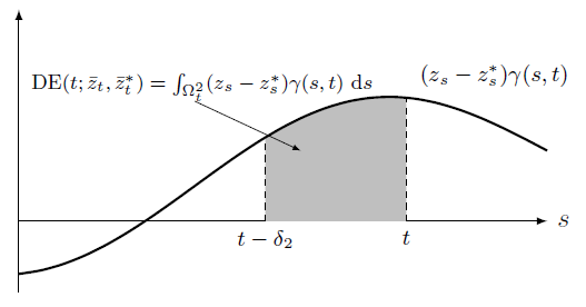
Direct Effect
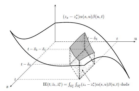
Indirect Effect
Causal effects are 1D/2D integration of the shaded
Method: Basis
- We estimate two SEM equations separately. The concurrent model is easy.
- Using the matrix form, $X = (M, Z)$, the historical model $$ Y(t)=\int_{\Omega_{t}} X(s)\theta(s,t)~\mathrm{d}s+\epsilon(t), $$
- Bivariate function $\theta_{j}(s,t)$ expanded as $$ \theta_{j}(s,t)=\sum_{k=1}^{K_{1j}}\sum_{l=1}^{K_{2j}}g_{klj}\phi_{kj}(s)\eta_{lj}(t) $$
- Solve the weighted regularized fitting criterion Ramsay, 2006, Wang et al, 2016 $$\scriptsize \mathrm{LMSSE}(\theta)=\int_{0}^{T}\| Y(t)-\mathbf{D}(t) \mathbf{G} \|_{2}^{2}~\mathrm{d}t+\lambda_{s}\mathrm{PEN}_{s}(\theta)+\lambda_{t}\mathrm{PEN}_{t}(\theta), $$ $$\scriptsize \mathbf{G}=\begin{pmatrix} \mathrm{vec}(\mathbf{G}_{1}) \\ \vdots \\ \mathrm{vec}(\mathbf{G}_{q}) \end{pmatrix}, ~ \mathbf{D}(t)=\begin{pmatrix} \boldsymbol{\eta}_{1}^\top(t)\otimes X_{1}^{*}(t) & \cdots & \boldsymbol{\eta}_{q}^\top(t)\otimes X_{q}^{*}(t) \end{pmatrix} $$
- The smoothness penalty $$\scriptsize \begin{align} \mathrm{PEN}_{s}(\theta) =& \int_{0}^{T}\int_{0}^{T}\{\mathcal{L}_{s}\theta(s,t)\}\{\mathcal{L}_{s}\theta^\top(s,t)\}~\mathrm{d}s\mathrm{d}t \end{align} $$
- Select $\lambda$ by cross validation
- Solve $ \mathbf{G}$ explicitly
Simulations
Simulations
- Compare with two other popular scalar methods:
- KKB: extension of Baron and Kenny for multilevel data
- Beta-KKB: summarize functions by feature vectors and then apply standard mediation
- These methods produce constant causal effect estimates
- Performance metrics include integrated MSE, MAE, and Bias
- Simulate from a functional mediation model with different sample sizes
Comparison
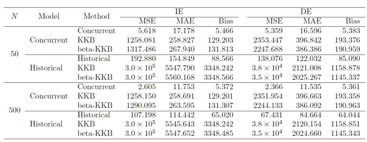
Challenging for scalar mediation methods to capture functional causal effects
Curve Estimation
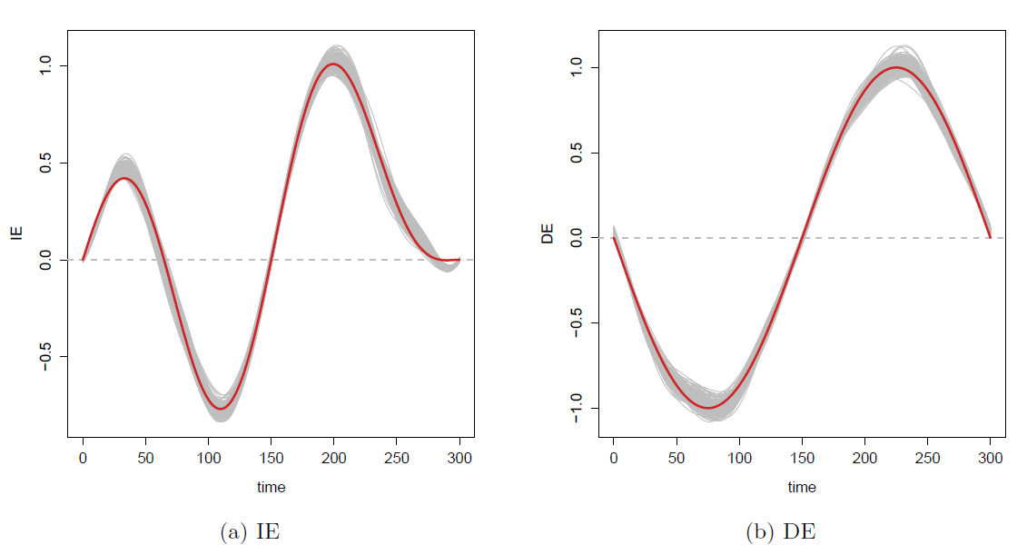
Estimated curves (gray) closely track the true curves (red)
Real Data
- N=121 subjects responding to the instructions of pressing and not pressing buttons while their brain activities were scanned by fMRI
- Two causal paths
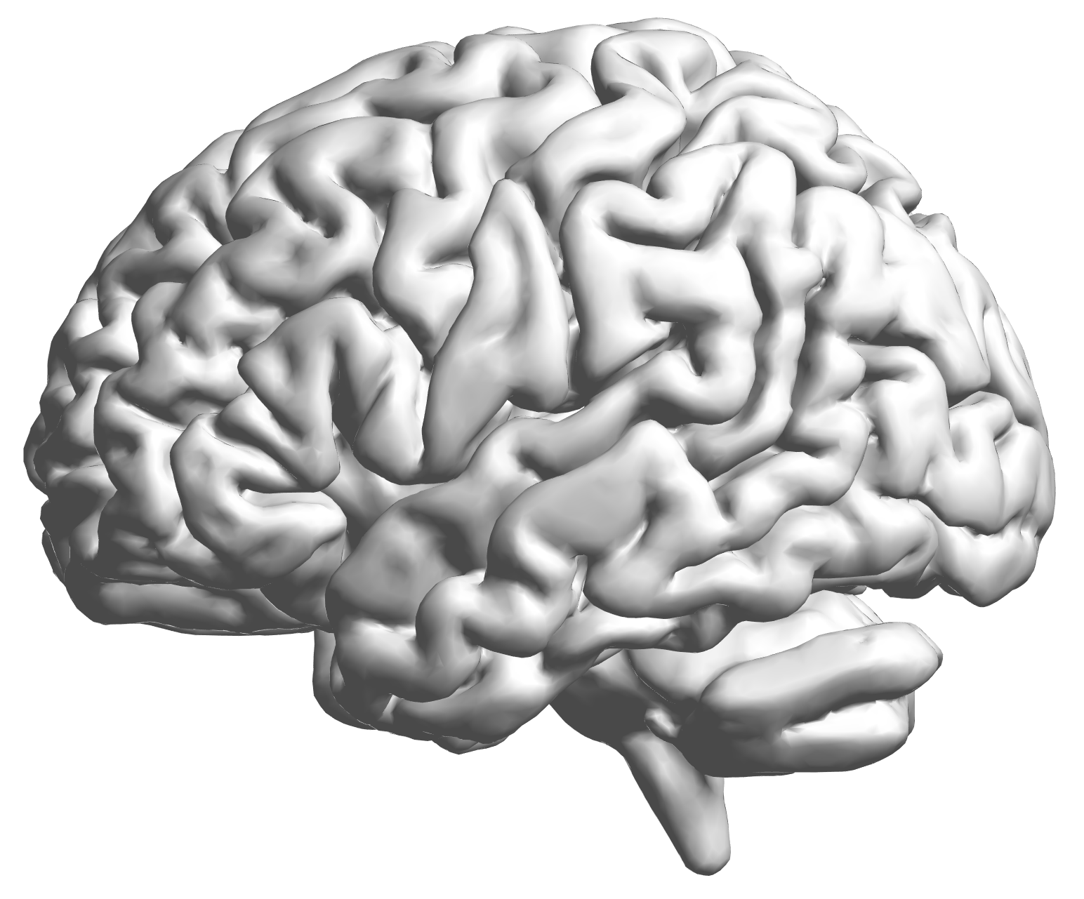
- IE: stimulus → preSMA brain region → M1 brain region
- DE: stimulus → M1 brain region
- We choose the tuning parameters, smoothness and historical window size, by cross-validation
- Inference is through bootstrapping, point-wise confidence bands
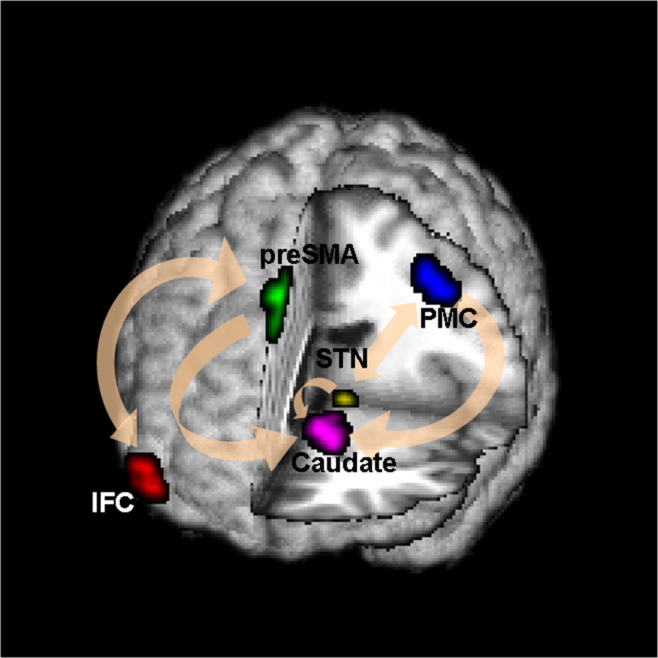
Brain Mediation Model
Goal: quantify functional
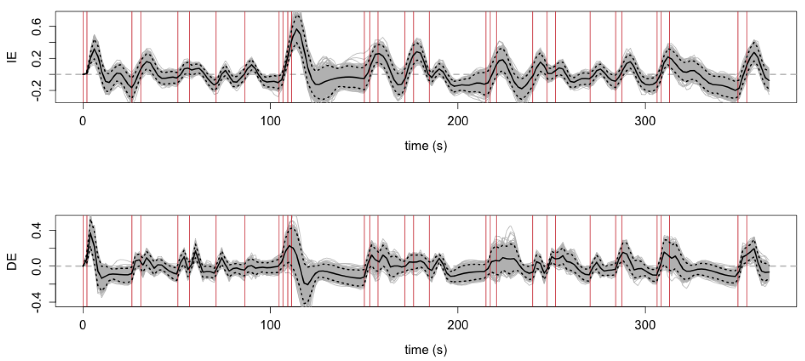
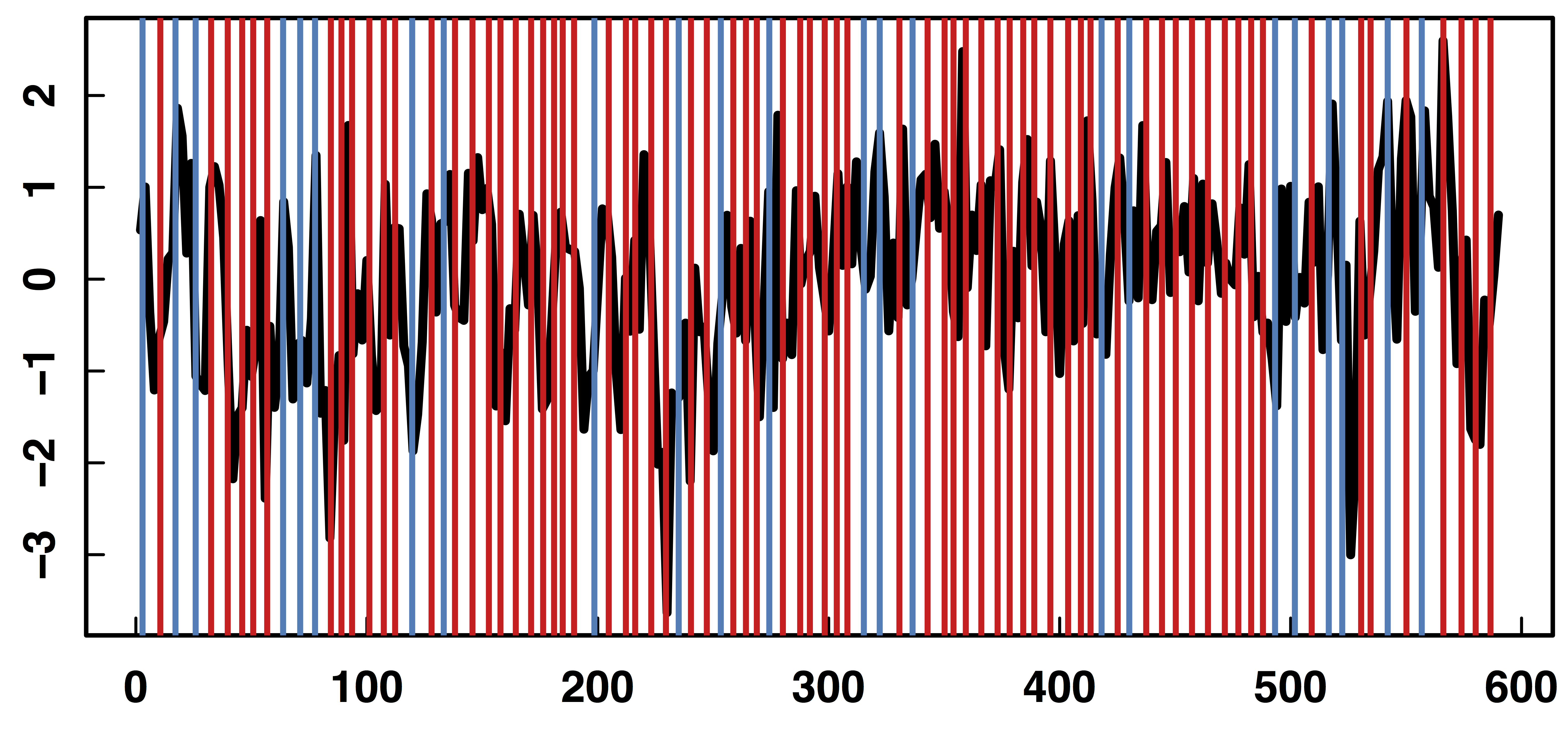
- Red vertical bars: stimulus instructions of withholding from pressing buttons
- Elevated IE/DE (solid lines) after the stimuli, especially when multiple stimuli presented in a short period prior
- Shaded areas: 95% point-wise confidence bands
Summary
- Functional model for mediation analysis
- Causal assumptions for identifiable effects
- Estimate dynamic causal effects as functional curves
- Enhance understanding of how the brain processes stimulus infomation
- R package available:
cfma
Thank you!
Comments? Questions?
BigComplexData.com
or BrainDataScience.com